DIRSIG includes a mechanism to define volumetric objects such as clouds and plumes that exist within the atmosphere using the OpenVDB voxel description.
These capabilities are not built directly into the DIRSIG5 model itself. Instead, a cloud or plume description is provided by a plugin and the local optical properties and temperatures are provided at run time (either calculated on-the-fly or pre-generated and sampled). The radiometry is handled by DIRSIG itself, calculating the emitted, scattered and transmitted (background) radiances. Note that depending on the type of model, environmental parameters such as the wind speed and direction can be obtained from the larger simulation environment.
Sources of VDB Files
Software
Since OpenVDB is a common file format used in the computer graphics community, VDB files can be created using a variety of tools. Below is a short list:
Pre-Generated
It should also be noted that there are collections of pre-generated VDB files available for free and for charge from various sources (e.g., use your favorite search engine to find results for "vdb cloud pack". As with all 3D assets (free or for charge), you must note the license accompanied by these assets, which sometimes limit usage of the asset to an individual and forbid sharing it with others. For example, Disney Animation Studios has made this collection of clouds available for free under the Creative Commons AttributionShareAlike 3.0 (CC BY-SA 3.0) license, which permits further sharing and adapting of the asset as long as you give credit to the original creator and share derived assets under the same license terms.
Shared Capabilities
Clouds and plumes are defined in the JSIM file as a
medium with the type set to either Cloud or Plume and with the
corresponding plugins defined in the respective plugin_list object.
Each JSON object in the respective plugin_list follows the same format
as the primary simulation plugins, with
a name defining which plugin is requested and an input object that
contains the input parameters for that plugin instance. Each plugin_list
can contain multiple plugin instances so that multiple clouds or plumes
can be defined.
"medium_list" : [
    {
        "type" : "Cloud",
        "plugin_list" : [
            {
                "name" : "CloudVDB",
                "inputs" : {
                    ...
                }
            }
        ]
    },
    {
        "type" : "Plume",
        "plugin_list" : [
            {
                "name" : "PlumeVDB",
                "inputs" : {
                    ...
                }
            }
        ]
    }
]
The OpenVDB-driven cloud and plume plugins share a common core that supports how VDB files are supplied, positioned, scaled, etc. The plugins assume the VDB contains one or two density, or "fog" grids that describe:
-
the concentration of the plume in parts per million [ppm] (or arbitrary concentration units if the dependent IOPs match)
-
the temperature of the plume in Kelvin [K] (the temperature is optional, but no emission will be calculated if it does not exist)
In the case of describing both properties, the grids exist in the same file and are not required to define the same voxelization. Each file represents a single temporal instantiation of the plume (i.e. it is instantaneous).
Common Input Parameters
The following input parameters are shared by both the cloud and plume plugins:
input_filename(required)-
This is the name of the actual OpenVDB file (or file sequence, as described below) that contains the concentration and, optionally, the temperature grids.
|
|
DIRSIG will check for the presence of every file in a given sequence before starting the simulation (to derive an overall bounding volume) and each frame must be provided in unit steps. |
resolution(optional)-
Voxel units in the OpenVDB file are assumed to be in meters (i.e. one step in index in any direction is a spatial change of one meter) unless a specific resolution is provided. Scaling is done before any other transformations are applied. Note that it is only possible to uniformly scale XYZ. The default resolution is
1meter. There are a discrete set of resolutions supported by the cloud and plume plugins:-
The
CloudVDBplugin supports the following:0.5,1.0,2.0,5.0or10.0meter resolution. -
The
PlumeVDBplugin supports the following:0.1,0.25,0.5or1.0meter resolution.
-
frame_delta(optional)-
If a sequence of VDB files is provided (a temporally dynamic scenario) then this parameter defines the time interval in seconds between each VDB "frame". The default frame delta is
1second. scale_concentration(optional)-
It is possible to scale the concentration values found in the OpenVDB file by an arbitrary amount. This may be useful, for instance, to change the effective units of concentration to match a new set of optical properties. The default concentration scale is
1. disable_interpolation(optional)-
This boolean variable will disable spatial interpolations within the VDB. The default value for this flag is
false. use_concentration_distance_cache(optional)-
This flag controls if a cache of concentration distance values is computed for each voxel to the sun. When not enabled, these values are computed (and potentially re-computed) on-the-fly. When enabled, during any temporal state change the values will be pre-computed for all voxels and saved. Enabling this feature can save time when modeling large, framing array sensors. However, it can slow down simulations using smaller arrays with frequent temporal state changes (e.g., pushbroom array type systems). The default value for this flag is
false.
VDB Sequences
A temporally static (constant) cloud or plume is represented by a single OpenVDB file.
"input_filename" : "example.vdb",A temporally dynamic (varying) cloud or plume is described via a
sequence of OpenVDB files representing the plume state at constant
time intervals. Each individual file is no different from a static
description and all of the concentration dependent optical properties
are shared between frames. The sequence is indicated by an indexing
convention in the filename that uses a fixed width, zero-padded
value (the width is arbitrary and only needs to be wide enough to
cover the number of frames being used, e.g. a width of two if the
indexes are always less than 100, a width of 4 if the indexes are
greater than 999. For example, a set of 15 .vdb files should be
named as follows:
frame00.vdb
frame01.vdb
frame02.vdb
...
frame14.vdb
|
|
Note the "frame" portion of the above filenames is just an
example. Text can be included before or after the frame numbers
in the filenames as long as it is the same in all files being
used.
|
When providing a dynamic cloud/plume, the filename incorporates a range of frame indexes into the filename (the first frame coincides with the start of the simulation regardless of the index numbers). The format is:
"input_filename" : "frame[00:14].vdb",It is also possible to only use a subset of indexes, where the first
index used corresponds to the start of the simulation. If the default
time delta between frames of 1 second is used, we can tell DIRSIG to
start with frame 05 and cover a 5 second sequence with the following
syntax:
"input_filename" : "frame[05:10].vdb",If a different inter-frame time delta is desired, then the
frame_delta parameter can be used.
|
|
If the simulation is querying the VDB sequence for a time between
the supplied frames, then the grids are linearly interpolated.
For example, if a 150 file sequence starts with an index of 0000,
the frame_delta is 1 second and a sensor is collecting at
time = 90.3 seconds, then the grid between the 91st (0090)
and 92nd (0091) VDBs are interpolated.
|
Static Positioning
For positioning a statically positioned cloud or plume, the user can provide a sequence of 3D translations and rotations:
translate(optional)-
The VDB can be translated from its native location (as stored in the VDB) by providing an optional translation in meters. This is supplied via a 3-element JSON array (e.g.,
"translate" : [ 10, 20, 30],). rotate(optional)-
The VDB can be rotated around its native origin by providing a set of Euler rotation angles in radians that are evaluated in Z, the Y, then X order. This is supplied via a 3-element JSON array (e.g.,
"rotate" : [ 0, 1.5707, 0],).
|
|
All translation and rotation transformations are performed in the order that they are given and multiple rotations and translations may be provided. |
Dynamic Positioning
The cloud or plume can be dynamically positioned using either the GenericMotion model or by supplying a velocity vector:
ppd_filename(optional)-
This variable specifies the name of the GenericMotion platform position data (PPD) file that describes the VDB’s location and orientation as a function of time (e.g.,
"ppd_filename" : "./geometry/cloud_motion.ppd"). velocity_vector(optional)-
This vector specifies the velocity as a 3-element JSON array in meters/second (e.g.,
"velocity_vector" : [ 0, 100, 0 ],).
The CloudVDB Plugin
The CloudVDB plugin allows the user to define a volumetric cloud
using the OpenVDB voxel description.
Optical Properties
This plugin currently utilizes a built-in database of cloud optical properties using data compiled by the team that develops the htrdr Monte-Carlo radiative transfer simulator. Specifically, from their atmosphere starter pack, which includes data for liquid water content, extinction, scattering phase functions, etc.
htrdr model.|
|
The ability for the user to provide their own extinction, scattering and phase function data will be added at a future date. |
Configuration
In addition to the shared OpenVDB parameters described previously, this plugin supports the following parameters:
override_temperature(optional)-
Sometimes it’s useful to fix the temperature of the cloud for testing purposes. If provided, the override temperature (Kelvin) will be used instead of whatever is in the OpenVDB grid or define the temperature for a VDB file that doesn’t contain a temperature grid.
medium_list object."medium_list" : [
{
"type" : "Cloud",
"plugin_list" : [
{
"name" : "CloudVDB",
"inputs" : {
"input_filename" : "cloud.vdb",
"translate" : [30,0,0],
"rotate" : [0,0,30],
"resolution" : 2.0,
"use_concentration_distance_cache" : true
}
}
]
}
],The PlumeVDB Plugin
The PlumeVDB plugin allows the user to define a volumetric cloud
using the OpenVDB voxel description.
A "plume" in DIRSIG is used to refer to a column of released
material being dispersed into another medium as it is acted upon
by the environment (e.g. the wind and surrounding air temperature).
Optical Properties
Spectral Absorption and Scattering
The optical properties description is provided in an external text file that gives the wavelength or wavenumber, the concentration dependent absorption coefficient and (optionally) the concentration dependent scattering coefficient. The spectral units are assumed to be wavenumbers, unless an optional [units] header is provided, e.g.
3700.000000	4.019800e-02
3699.500000	1.237900e-02
3699.000000	5.621300e-03
3698.500000	3.779900e-03
3698.000000	2.733500e-03
3697.500000	2.178500e-03
3697.100000	1.772400e-03
3696.600000	1.508800e-03
3696.100000	1.294800e-03
...
describes the absorption (only) as a function of wavenumbers, while:
[microns]
2.600000 1.957900e-04  1.649700e-03
3.100000 2.048500e-04  1.817000e-03
3.600000 2.139700e-04  1.997900e-03
4.000000 2.241600e-04  2.293100e-03
4.500000 2.344500e-04  2.651600e-03
...
describes both absorption and scattering as a function of the wavelength in Microns. The general format is:
([units])
[spectral point] <del> [absorption coefficient] <del> ([scattering coefficient])
...
Where:
-
the delimiter (
<del>) can be any amount of whitespace and/or a comma -
the optional spectral units can be [wavenumbers], [nanometers], or [microns]
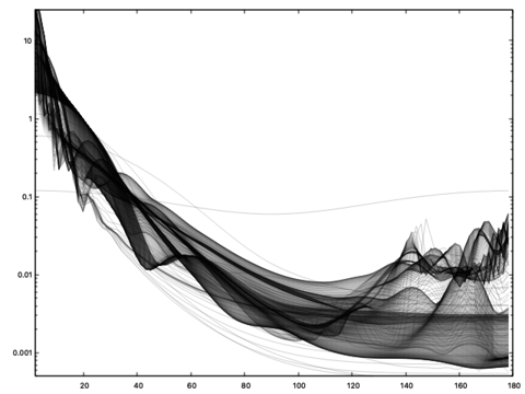
Scattering Phase Functions
If scattering coefficients are provided then it is expected that a file will be provided that describes the scattering phase function (assumed rotationally symmetric around the forward direction). If one isn’t provided then nominal water vapor characteristics will be used.
The scattering phase function (SPF) is dependent both on the angle (as measured from the forward direction) and on the wavelength being modeled. As such the SPF file is structured as:
[list of SPF wavelengths separated by <del> and given in µm]
[0] <del> [N SPF values separated by <del> (N = number of wavelengths)]
[angle (deg)] <del> [N SPF values and separated by <del> (N = number of wavelengths)]
...
[180] <del> [N SPF values and separated by <del> (N = number of wavelengths)]
where the 0 and 180 degree entries are mandatory and other
angles should be given in increasing order (note that they do not
have to be regularly sampled).
Configuration
The concentration of the plume is not sufficient for describing it’s optical properties and the corresponding absorption and scattering coefficients are calculated by giving the model concentration dependent spectral descriptions with units of inverse [ppm m] such that the final absorption and scattering coefficients have units of [1/m]. Note that any particular combination of concentration and dependent optical properties could be used as long as they are consistent.
All files are assumed to be specified with either absolute paths or relative to the folder in which the simulation is being run.
In addition to the shared OpenVDB parameters described previously, this plugin supports the following parameters:
ext_filename(required)-
This is the name of the file that collectively describes the optical properties for extinction in the plume: the spectral absorption and, optionally, the spectral scattering (see above).
spf_filename(optional)-
If the extinction file above has a spectral scattering column then it is possible to provide a file describing the spectral scattering phase function (see above).
The plume plugin follows the basic plugin definition described in
the JSIM manual, but in the context of
the medium list. Multiple plumes can
be incorporated into a simulation by supplying multiple plume entries
in the Plume type object in the medium_list:
medium_list object."medium_list" : [
{
"type" : "Plume",
"plugin_list" : [
{
"name" : "PlumeVDB",
"inputs" : {
"input_filename" : "plume1.vdb",
"ext_filename" : "gas.txt",
"translate" : [30,0,0],
"rotate" : [0,0,30]
}
}
]
},
{
"type" : "Plume",
"plugin_list" : [
{
"name" : "PlumeVDB",
"inputs" : {
"input_filename" : "plume2.vdb",
"ext_filename" : "gas.txt",
"translate" : [-1,0,-10],
"rotate" : [0,0,0]
}
}
]
}
],However, overlapping the active areas of the voxelizations will likely not result in appropriate behavior and should be avoided as much as possible. The interaction of multiple plumes with the same optical properties, such as passive mixing or the collision of turbulent material, should be modeled externally and provided in the same VDB file.
Plumes with multiple materials
It is possible that a single plume contains multiple materials that do not exist throughout the volume in the same proportion to each other. In that case, it is not sufficient to describe the optical properties with a single concentration for each voxel and a single set of concentration-dependent absorption and scattering coefficients. Instead, DIRSIG allows for multiple concentration values in the VDB definition, facilitating the simultaneous definition of 2 or 3 different materials.
To define multiple (2 or 3) materials in a single plume voxelization,
the concentration portion of the OpenVDB file must be generated
using the vec3s data type (i.e. a 3-element vector of "float"
values for each voxel) instead of the usual "float" data type.
The temperature portion of the VDB file (if used) does not change and continues to be based on a scalar "float". If two materials are being defined, then only the first two elements of the vector should be set for each voxel (the third will be ignored) and all three should be used in the case of three materials.
The number of materials in a plume is indicated to DIRSIG by the number of concentration-dependent optical properties that are provided using a JSON array rather than a single filename for each. For example, to define three absorbing materials, the plugin definition might look like:
"medium_list" : [
    {
        "type" : "Plume",
        "plugin_list" : [
            {
                "name" : "PlumeVDB",
                "inputs" : {
                    "input_filename" : "mixed3.vdb",
                    "translate" : [0,0,0.5],
                    "rotate" : [0,0,0],
                    "resolution" : 1.0,
                    "scale_concentration" : 1,
                    "ext_filename" : ["cyan.abs","magenta.abs","yellow.abs"],
                    "disable_interpolation" : true
                }
            }
        ]
    }
],
This "plume" is made up of three different materials that absorb light in different areas of the visible spectrum (mimicking the subtractive primaries of common printer inks). The corresponding "mixed3.vdb" defines volumes where the materials exist on their own or overlap with one or both of the other materials.

A plume definition with only two materials would only have two files in the "ext_filename" array and adding scattering uses the same array format for the scattering phase function file names.
Example Outputs
Spectral Radiance Imagery
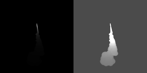
The following nadir viewing image is generated by the PlumeOpenVDB1 demo using an SF6 gas. The wavelength being visualized corresponds to the main absorption feature of SF6 and demonstrates both emission and absorption modes as the plume is released and cools off away from the stack.
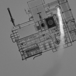
PlumeOpenVDB1 demo.Relevant Truth Products
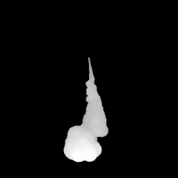
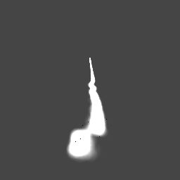
Information about the plume can be extracted from the simulation through the use of truth outputs. The plethora of plume-specific truth products available in DIRSIG4 are not readily available via the plugin approach used in DIRSIG5, but there are still many options available. In particular, the intersection truth can give information about the boundary of the plume itself (the "hit" as a path encounters the volume).
|
|
The outer boundary of the voxelization corresponds to any active voxels regardless of their content. If the VDB you are using has many low valued concentrations, the boundary shown in the truth will likely be much larger than the "visible" plume in a render. |
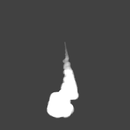
The intersection truth products are described here. The recently introduced medium intersection truth products report the respective coordinate of a boundary inside the plume (e.g., an object inside the plume) or the coordinate of the exit boundary.
Other standard truth values have been updated to provide information about a plume as well:
|
|
Many of the truth products are based on the primary path through the plume (i.e. before a solid object is encountered). If the plume incorporates scattering, then the truth values are based on the wandering (not straight) path taken through the volume, averaged over all the path samples. |
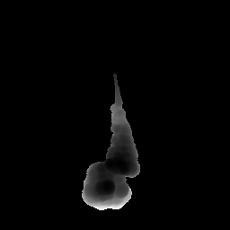
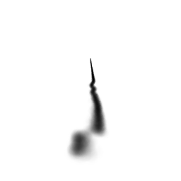
Finally, if you want to know the average actual path length traveled in the volume, a new truth product has been added called volpathlength. This truth collector provides the average path length traveled within the first volume encountered (not including the atmosphere). If the path exits the plume and re-enters, only the first traversal will be included. Since the plume below does not scatter, the path length truth corresponds directly to the difference between the two intersection truth products above.
volpathlength truth product.